Note: This post was published on DZone.
TL;DR:
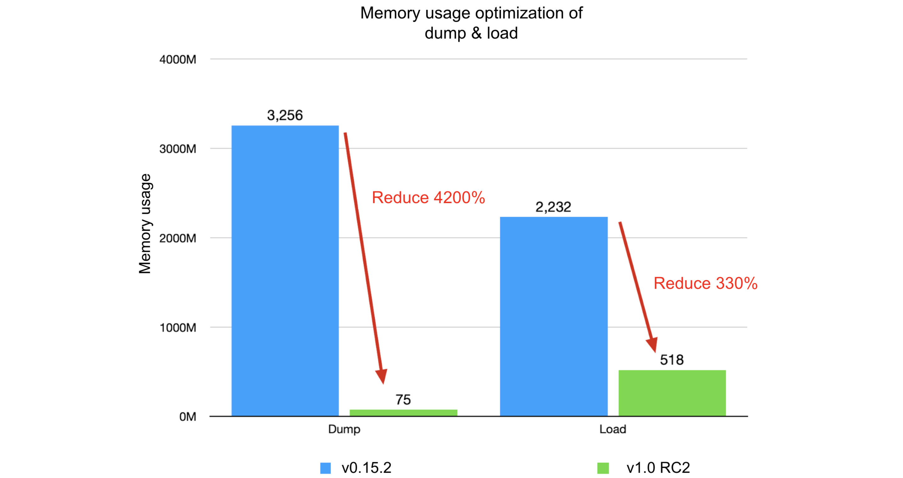
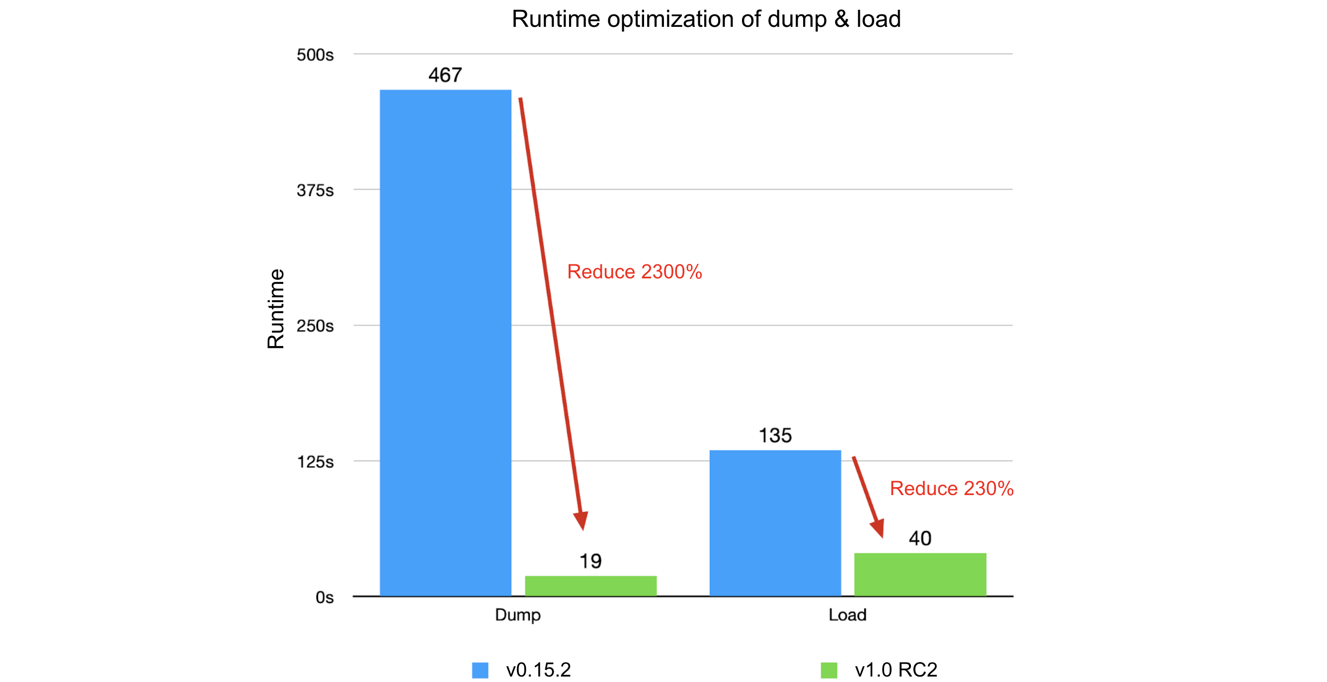
JuiceFS achieved a 40x performance boost in metadata backup and recovery through optimizations from v0.15.2 to v1.0 RC2. Key optimizations focused on reducing data processing granularity, minimizing I/O operations, and analyzing time bottlenecks. The overall improvements resulted in a 2300% reduction in dump process runtime and a 4200% decrease in memory usage, while the load process achieved a 230% runtime reduction and a 330% decrease in memory usage.
As an open-source cloud-native distributed file system, JuiceFS supports various metadata storage engines, each with its unique data management format. To facilitate management, JuiceFS introduced the dump command in version 0.15.2, allowing the uniform formatting of all metadata into a JSON file for backup. Additionally, the load command enables the restoration or migration of backups to any metadata storage engine. For details on these commands, see Command Reference. The basic usage is as follows:
$ juicefs dump redis://192.168.1.6:6379/1 meta.json
$ juicefs load redis://192.168.1.6:6379/2 meta.json
This feature underwent three significant optimizations from version 0.15.2 to 1.0 RC2, resulting in a 40x performance improvement. The optimizations primarily focused on three aspects:
- Reducing data processing granularity: Splitting large objects into smaller ones significantly reduced memory usage and allowed for fine-grained concurrent processing.
- Minimizing I/O operations: Employing a pipeline approach for batch requests reduced network I/O time.
- Analyzing time bottlenecks in the system: Shifting from serial to parallel processing enhanced CPU utilization.
These optimization strategies are quite typical and have broad applicability in scenarios involving numerous network requests. In this post, we’ll share our specific practices in the hope of inspiring others.
Metadata format
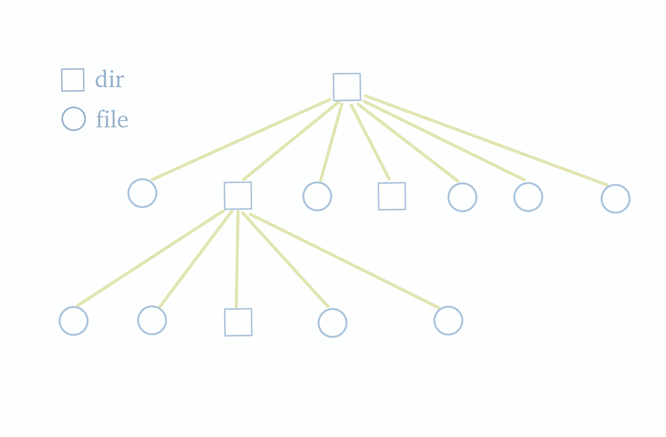
Before delving into the dump and load functionalities, let's first understand the structure of a file system. As shown in the diagram below, the file system follows a tree structure with a top-level root directory. The root directory contains subdirectories or files, and these subdirectories, in turn, may have their own subdirectories or files. Therefore, to obtain information about all the files and folders within the file system, we simply need to traverse this tree.
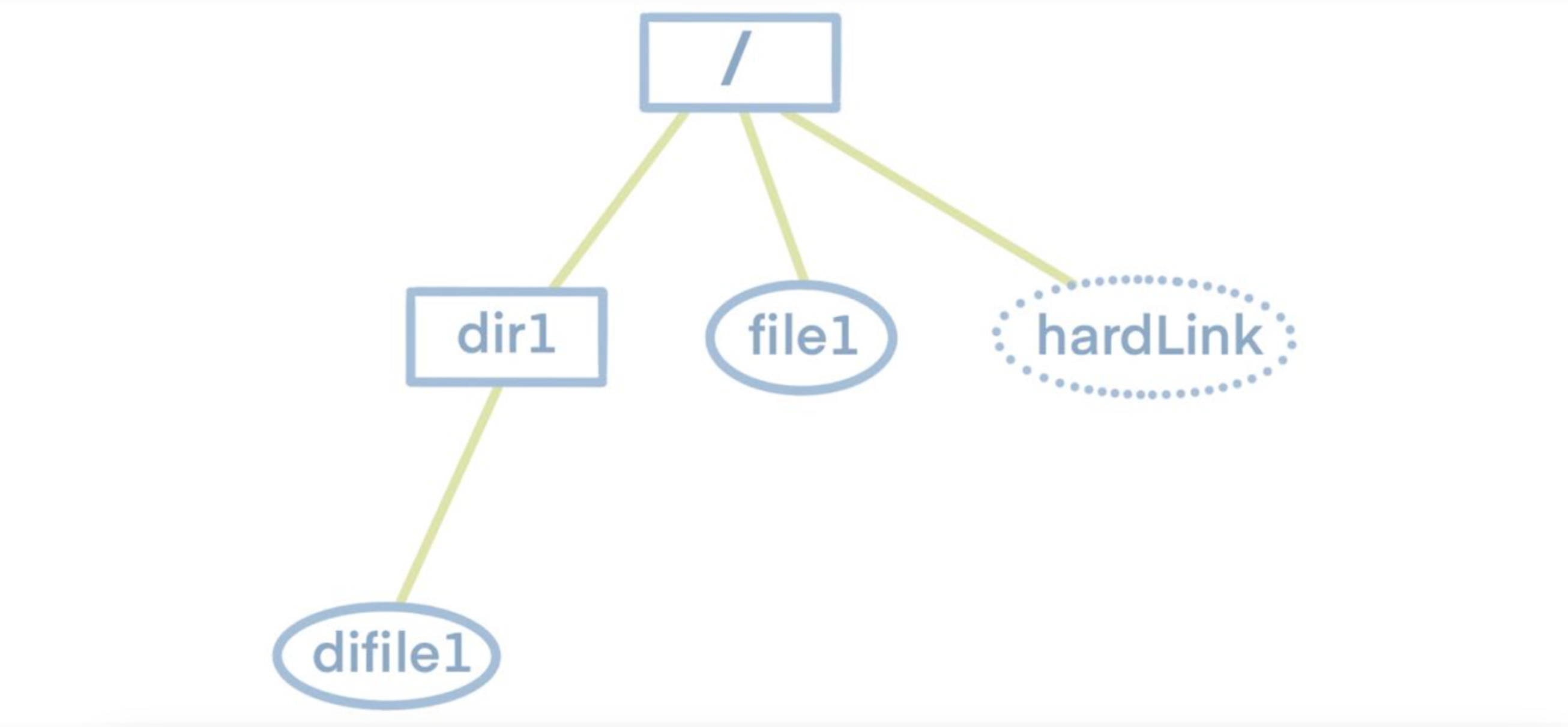
Knowing this, we can examine the characteristics of JuiceFS metadata storage. JuiceFS metadata storage primarily consists of several hash tables. Each table's key is the inode of a single file. The inode information can be obtained by traversing the file tree. Hence, by traversing the file tree to gather all inodes and using them as indexes, we can retrieve all metadata.
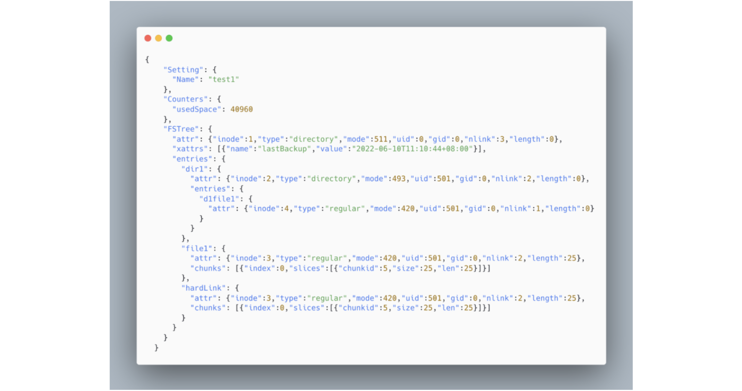
To enhance readability and preserve the original file system's tree structure, the export format is set as JSON. Below is an example of a JSON file dumped from the aforementioned file system, where hardLink denotes a file's hard link.
Optimizing the dump process
Before dump optimization
Implementation of dump
We implemented dump through the following steps:
1. Examining the metadata format reveals that all metadata uses the inode as a partial variable key. This implies that knowing the specific value of the inode allows us to retrieve all metadata information from Redis. Therefore, based on the file system's characteristics, we constructed an FSTree by performing a depth-first scan, filling this tree by scanning the root directory first (inode 1) and subsequently scanning all entries below it.
- During this process, if an entry was a directory, we recursively scanned it.
- Otherwise, we sent requests to Redis to retrieve various dimensions of its metadata, assembled the information into an entry structure, and included it in the parent directory's entry list.
After completing the recursive traversal, the FSTree was fully constructed.
2. We added relatively static metadata such as settings as an object and serialized the entire tree into a JSON string.
3. We wrote the JSON string to a file.
Performance
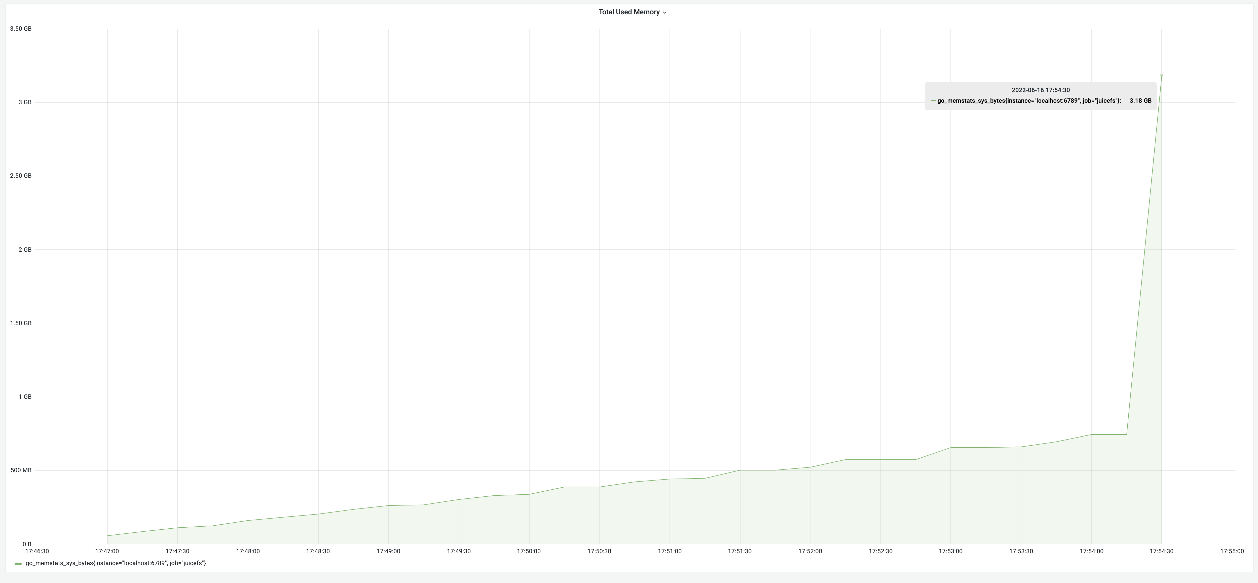
We took Redis containing 1.1 million files’ metadata as an example for testing. The test results showed that the dump process took 7 minutes and 47 seconds and the memory usage was 3.18 GB. Note that to ensure the comparability of test results, all tests in this article used the same metadata.
The test results:
- The memory usage initially rose slowly as each entry was scanned during the depth-first traversal.
- Once the entire FSTree object was constructed, the JSON serialization process began. The FSTree object was approximately 750 MB at this point. Serializing an object into a JSON string required about twice the object's size.
- Finally, the JSON string was roughly the size of the original object.
- As a result, the memory usage increased by about three times the size of the FSTree object, rapidly reaching 3.18 GB. The ultimate peak memory usage was estimated to require approximately four times the size of the FSTree.
Issues with the implementation above
The core of our approach was constructing an FSTree object. The JSON serialization method could directly serialize an object into a JSON format string. Therefore, once we built the FSTree object, the rest could be done by the JSON package, which was convenient.
For a file system with many large files, the metadata was substantial. FSTree saved the metadata information of the entire system's entries, so the memory occupied by the dump process would be high.
Additionally, after serializing the object into a JSON string, the string's size was large, essentially equivalent to twice the metadata size. If the client hosting the dump process lacked sufficient memory, the operating system might kill the process due to out-of-memory (OOM) issues.
Optimizing dump memory usage
How we reduced memory usage
To address the issue of high memory usage, we reduced the granularity of data processing. Instead of serializing the entire FSTree object, we split it into smaller objects and serialized each entry separately, appending the resulting JSON strings to the file.
We conducted a depth-first recursive scan of the FSTree.
- For each entry encountered, we serialized it and wrote it to a JSON file.
- If the entry was a directory, we recursed it.
Consequently, the resulting JSON file maintained a one-to-one correspondence with the FSTree object, preserving the tree-like structure and order of entries. This way, in the dump memory, we only retained an object with the size of metadata, resulting in a significant memory saving.
We also saved the remaining half of the memory by serializing and writing each entry to the JSON file as soon as it was constructed. By doing so during the entire file system traversal, all entries were serialized without the need to construct and store the entire FSTree.
Finally, we didn’t need to build the FSTree object, and each entry was only accessed once, serialized, and then discarded. This resulted in even less memory consumption.
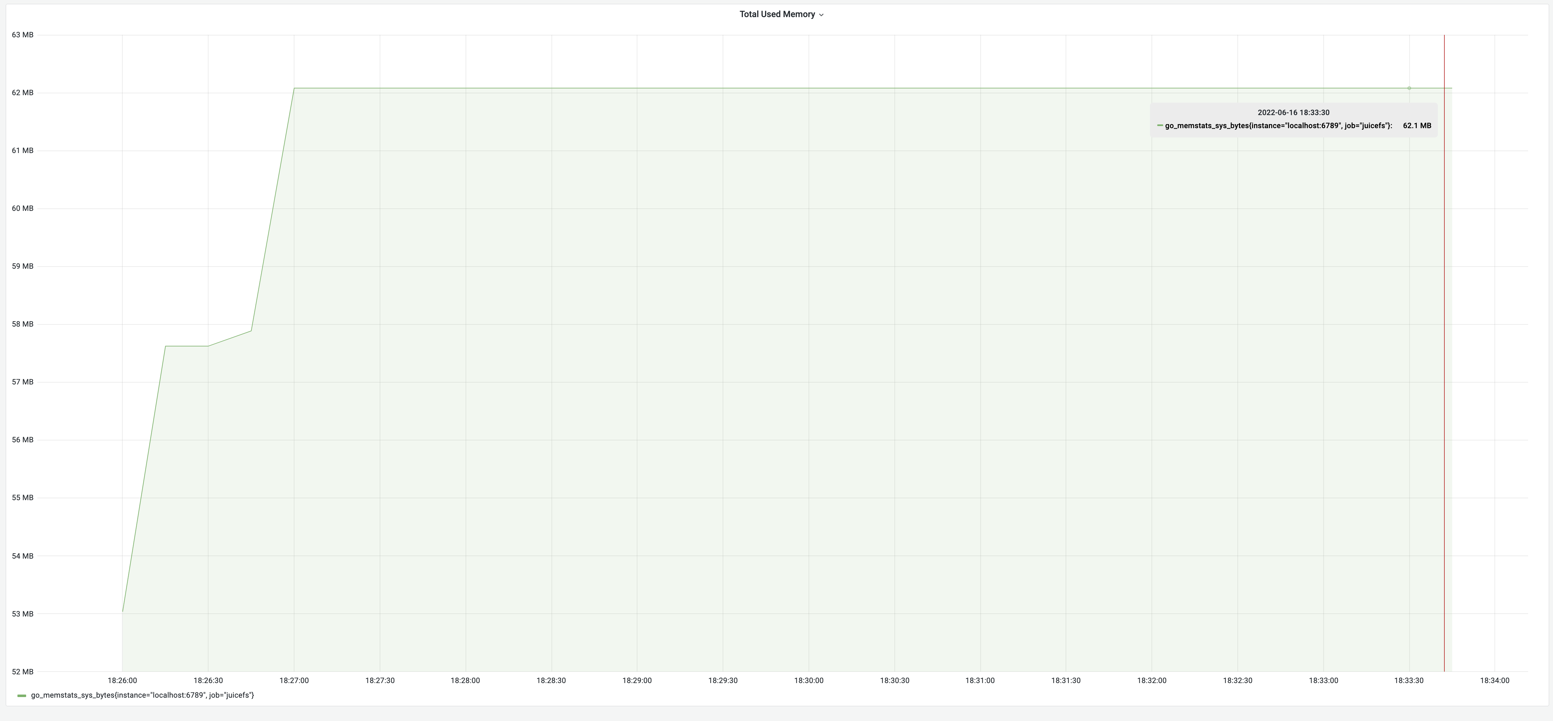
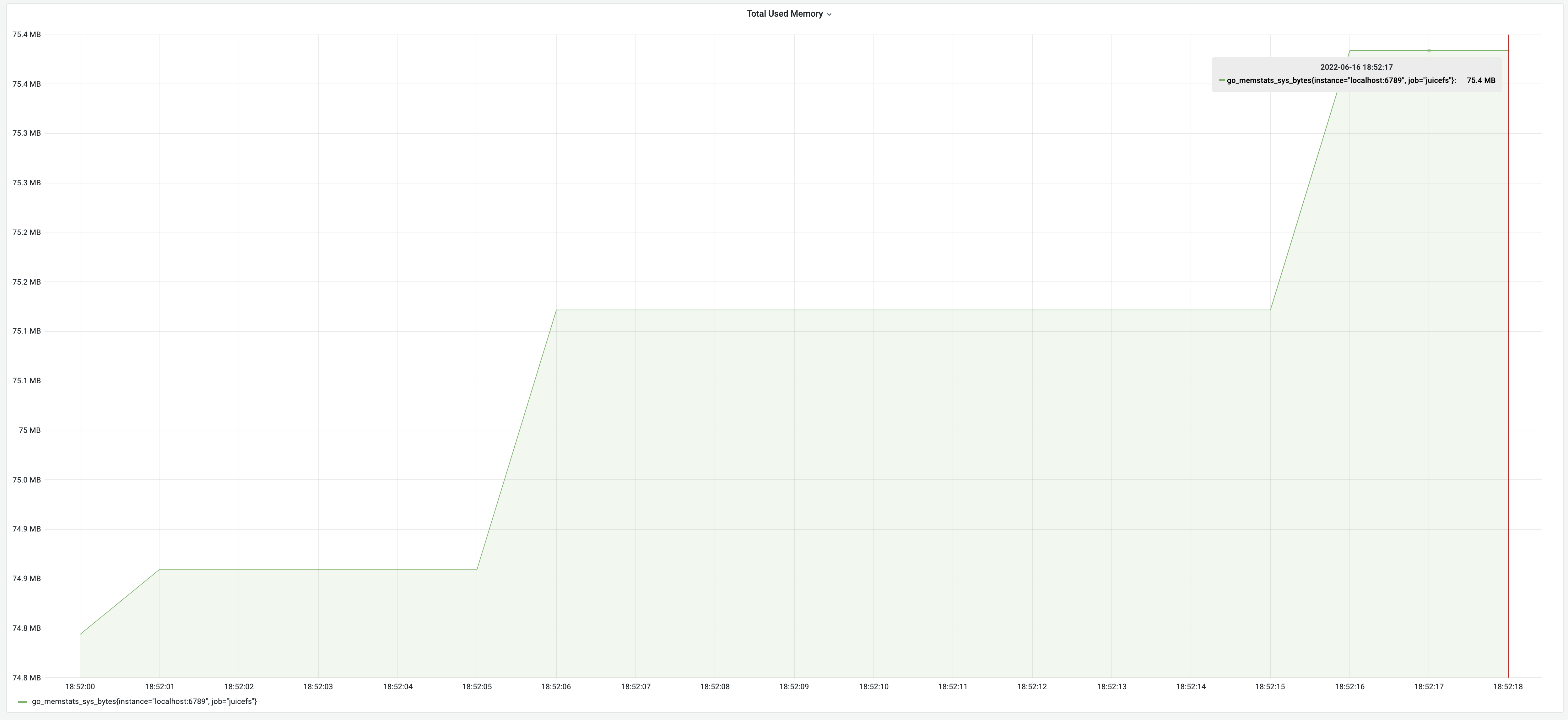
Performance after memory usage optimization
After memory usage optimization, the test results for the dump process were 8 minutes, with memory usage of 62 MB. Although the time consumption remained the same, the memory decreased significantly from 3.18 GB to 62 MB, achieving an impressive 5100% improvement! The memory usage changes are illustrated in the graph below:
Optimizing the dump runtime
How we optimized the dump runtime
From the above test results, one million dumps took about 8 minutes. If there were one hundred million files, it would take 13 hours. Such prolonged durations were unacceptable in production. While insufficient memory could be addressed with "throwing money at the problem," excessively long processing times diminished the effectiveness of this approach. Therefore, the solution required optimizing the internal program logic.
Let's analyze which step was consuming the most time.
Typically, time consumption can be categorized into two aspects:
- A significant number of computational operations
- Numerous I/O operations
In our case, it is clear that we were dealing with a large amount of network I/O operations. The dump process required a request for metadata information for each entry encountered, and each request's time consumption was composed of round-trip time (RTT) plus command calculation time. Redis, being in-memory, calculated commands quickly. So the primary time-consuming factor was the RTT. With N entries, there were N RTTs, leading to a substantial time cost.
To reduce the number of RTTs, we could use Redis' pipeline technology. The basic principle of a pipeline was to send N commands at once. Redis processed all N commands and returned the results to the client in one go, combining the results in the order of execution. Thus, the time cost for N commands was reduced to 1 RTT plus the time to compute N commands. In practice, the optimization achieved by using a pipeline was significant.
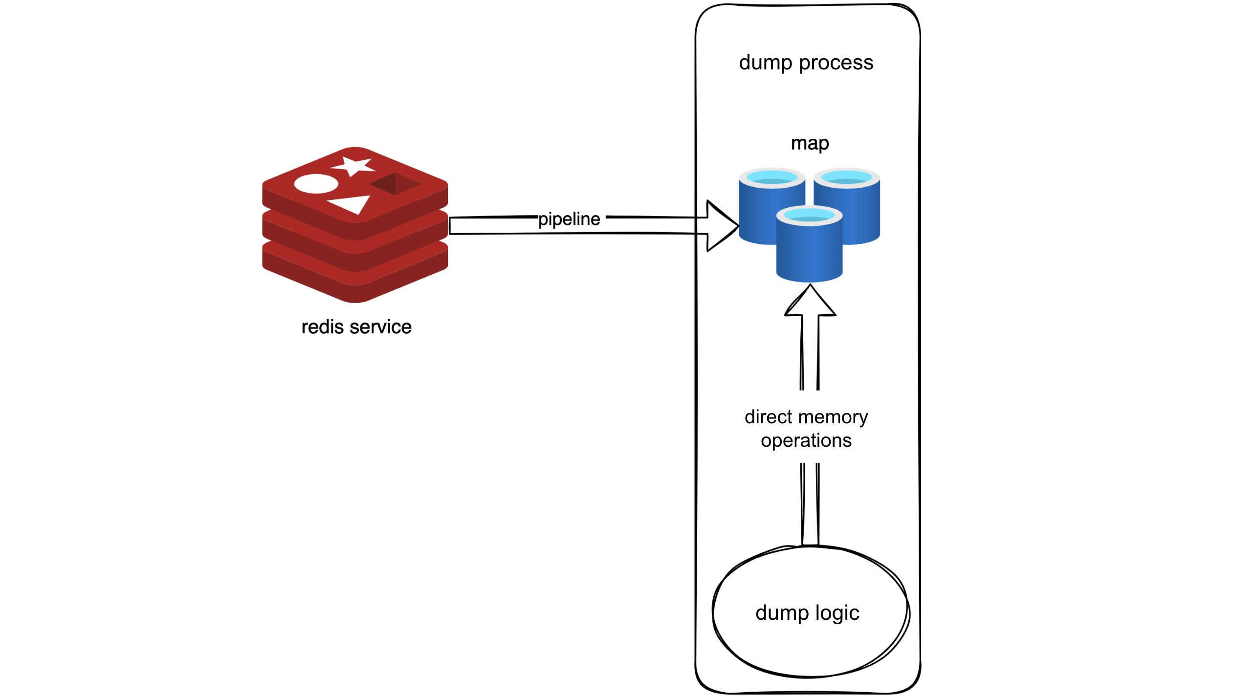
Following this logic, we used a pipeline to retrieve all metadata from Redis into memory. It was akin to creating a snapshot of Redis in memory. Code-wise, this involved placing the metadata into a map, effectively replacing the original logic that required Redis requests with reading from the map.
With this idea, we used a pipeline to fetch all metadata in Redis into memory, creating a sort of Redis snapshot in memory. In the code, this was implemented by storing the metadata in a map, allowing the original logic, which used to request data from Redis, to directly retrieve it from the map now. This approach leveraged the pipeline for bulk data retrieval, reducing RTTs, and required minimal changes to the original logic—simply replacing Redis request operations with map reads.
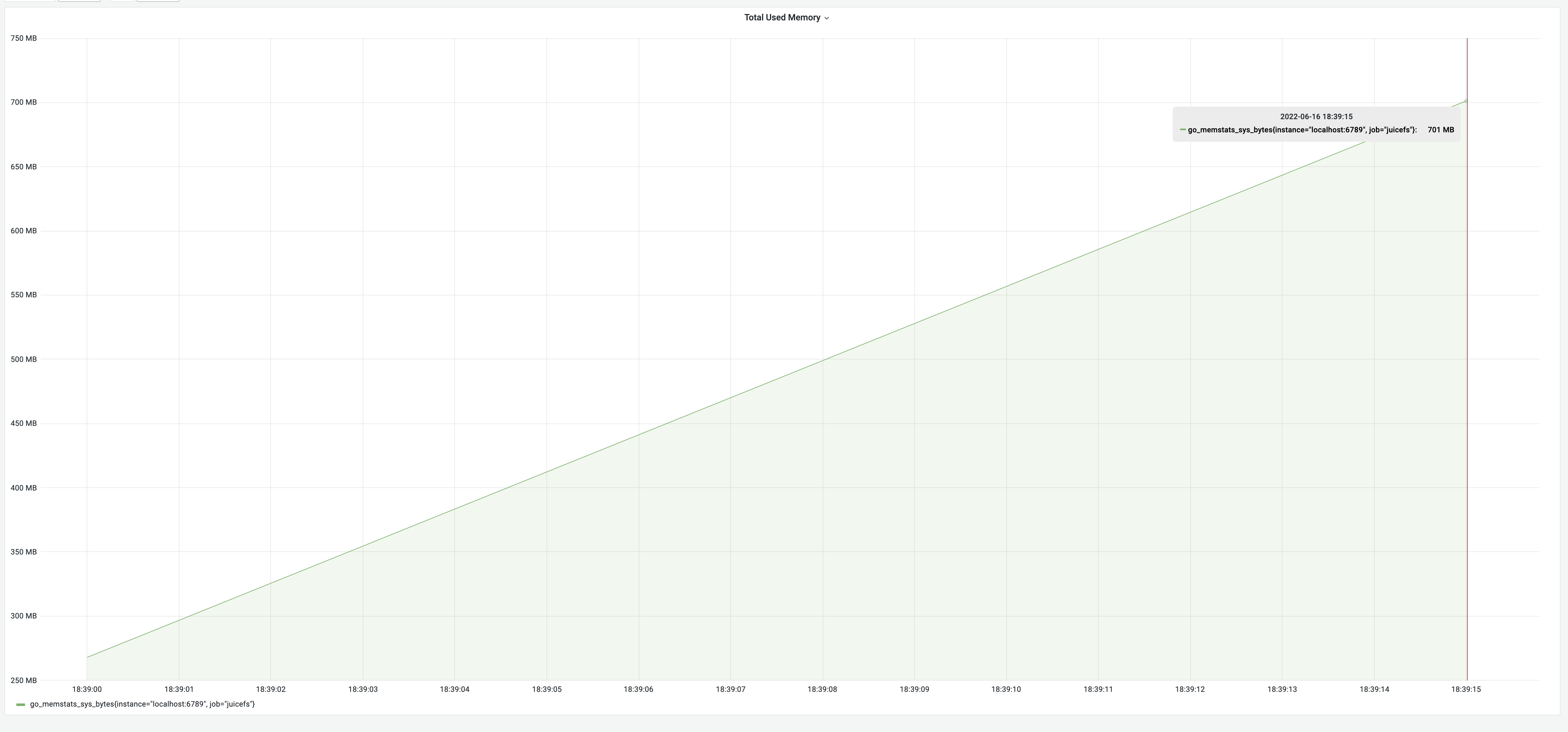
Performance after optimizing with the "snapshot" approach
After optimizing with the "snapshot" approach, the dump process took 35 seconds, with memory usage of 700 MB. The time consumption significantly decreased from 8 minutes to 35 seconds, a remarkable 1270% improvement. However, the memory usage increased to 700 MB due to constructing a metadata cache in memory, approximately the size of the metadata, as indicated by the earlier test results. This met our expectations.
How we achieved both low memory usage and runtime
While the "snapshot" approach improved speed considerably, it essentially placed all of Redis' data into memory. This resulted in high memory usage, essentially the size of the metadata. So, optimizing for time consumption sacrificed memory usage. The size of the memory usage and a long processing time were both unacceptable in production. Therefore, a compromise was needed.
Reflecting on the two previous optimizations: streaming writing addressed the high memory usage, and using Redis pipeline reduced the number of RTTs. Both optimizations were necessary, and the key was to combine them effectively.
Combining the pipeline with streaming writing to reduce memory usage
We considered adding the pipeline functionality to the streaming writing version. The streaming writing version could be seen as a pipeline process, where the source end was responsible for sequentially constructing entries, and the receiving end was responsible for sequentially serializing entries. The order of entries corresponded to the depth-first traversal order of the FSTree. To use a pipeline, we must go through batch processing. Therefore, we could logically divide entries into multiple batches, each with a length of 100. Each batch was a processing unit in the pipeline. The process became:
- The source end notified the receiving end to start serializing the batch after processing one batch.
- The receiving end notified the source end to construct the next batch after serializing the current batch.
- The steps above were repeated until completion.
Each batch used a pipeline to speed up getting results. This way, the pipeline and streaming writing coexisted. This was how we optimized memory usage.
Parallelizing the pipeline insertion to reduce runtime
We could also further optimize time consumption. We analyzed the current pipeline operation and found that when the source end sent a pipeline request for metadata, the receiving end was idle, as there was no data to serialize. Similarly, when the receiving end was serializing, the source end was idle. Therefore, the pipeline operated intermittently, resulting in serial computation. To further reduce time consumption, we parallelized the pipeline insertion to increase CPU utilization and speed up the process.
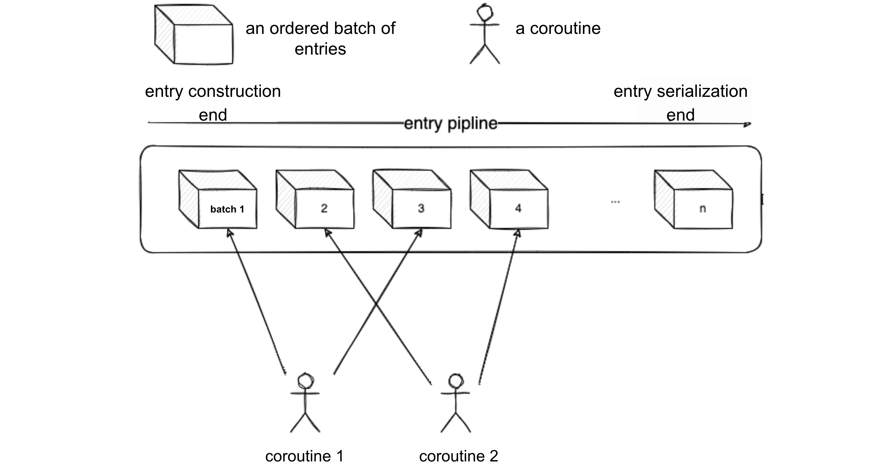
Next, we considered how to make the source end and the serialization end work in parallel. For the same batch, data generation and processing were certainly not parallelizable. Only batches with metadata not yet requested and batches to be serialized could be processed in parallel. In other words, the source end didn’t have to wait for the serialization end to finish. The source end just needed to fetch data, and the fetched data was placed on the pipeline in order. The serialization end serialized data in order.
If it found that a batch had not been fetched yet, it waited until the source end informed it that the batch was ready. Considering that the speed of batch construction was slower than the time it took to serialize a batch, we could also add concurrency to the source end. The source end simultaneously serialized multiple batches to reduce the serialization end's waiting time.
Let's visualize the process with the following diagram. Suppose the current concurrency level of the source end is 2.
- Coroutine 1 and Coroutine 2 simultaneously construct Batch 1 and Batch 2. Meanwhile, the serialization end is waiting for Batch 1 to be constructed. Once Coroutine 1 completes the construction of Batch 1, it notifies the serialization end to start serializing Batch 1 sequentially.
- When Batch 1 is serialized, the serialization end notifies Coroutine 1 to start constructing Batch 3. This is because Batch 2 and Batch 4 are handled by Coroutine 2, and each coroutine is assigned batches for the serialization end to deduce which one to notify next according to certain rules.
- After notifying Coroutine 1, the serialization end starts serializing Batch 2. It first checks if Batch 2 is ready; if not ready, Coroutine 2 is expected to notify.
- After serializing Batch 2, the serialization end notifies Coroutine 2 to start constructing Batch 4, and so on. This way, the serialization end can serialize entries in parallel with the source end processing entries, keeping up with the serialization speed.
The actual process of the above logic steps executed on a tree-structured file system is illustrated in the following diagram:
Performance after optimizing memory usage and runtime
After we optimized memory usage and time consumption, the testing results were a runtime of 19 seconds and a memory usage of 75 MB. This got the optimal effects of each individual optimization. It truly achieved the goal of getting the best of both worlds.
Optimizing the load process
Before load optimization
An infeasible method
Compared to dump, the logic for load was simple.
The most straightforward method was to:
- Read the entire JSON file into memory.
- Deserialize it into the FSTree object.
- Traverse the FSTree tree in depth-first order.
- Insert each entry's metadata dimensions into Redis separately.
However, this method had a problem. Taking the example of the file tree in the JSON file content mentioned earlier, there was a situation during the dump of this file system: file1 had already been scanned, and Redis returned nlink for file1 as 2 (because hardLink was hard-linked to file1). At this point, the user deleted hardLink, and nlink for file1 was modified to 1 in Redis. However, because it has already been scanned in the dump, the nlink in the JSON file dumped still remained 2, leading to an nlink error. nlink was crucial for the file system, and errors in its value could cause problems such as inability to delete or data loss. Therefore, this method that could lead to nlink errors was not feasible.
The solution
To solve this problem, we needed to recalculate the nlink value during load. This required us to record all inode information before loading.
- We built a map in memory, with the key being inode and the value being all the metadata of the entry.
- When traversing the entry tree, we put all scanned file type entries into the map instead of inserting them directly into Redis. Before entries were put into the map each time, the system checked whether this inode already existed. If it existed, it meant this was a hard link, and we needed to increment the
nlinkof this inode. The same situation might also occur on subdirectories. Therefore, traversing to a subdirectory required incrementing thenlinkof the parent directory. After traversing the entry,nlinkwas recalculated. - We traversed the entry map and inserted all the metadata of the entries into Redis. To speed up insertion, we needed to use the pipeline method.
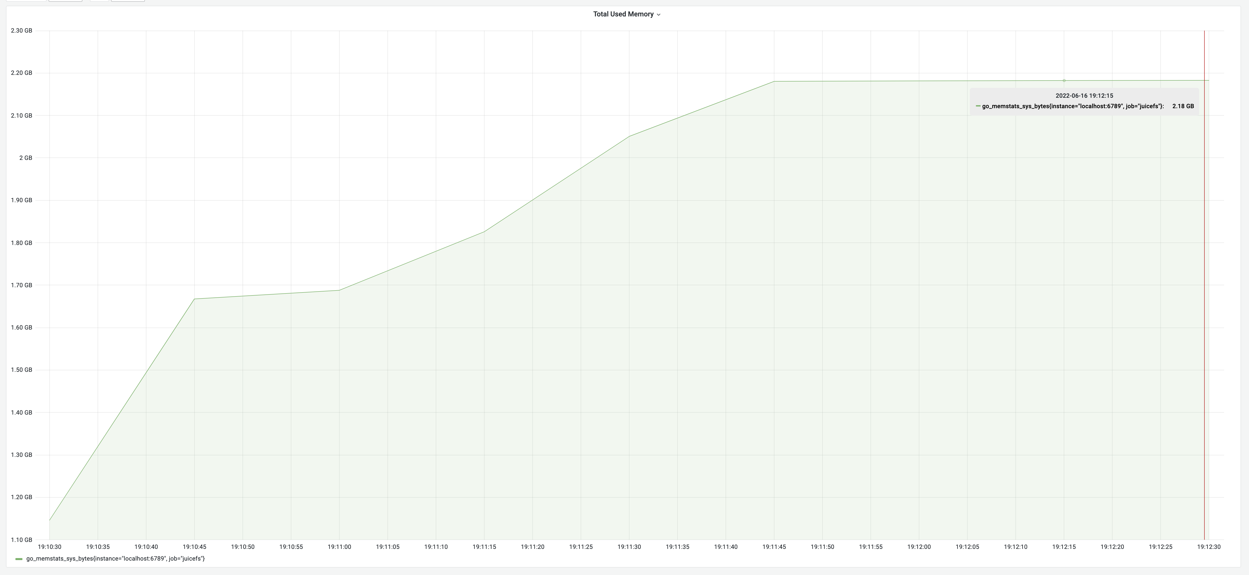
Performance based on the solution above
The testing result according to the above logic: a runtime of 2 minutes and 15 seconds, with a memory usage of 2.18 GB.
Optimizing load runtime
How we reduced load runtime
Just using a pipeline did not reduce the runtime to the extreme. We could further reduce the time through other methods. Redis was very fast, even if using a pipeline, the processing speed of commands was still much lower than the RTT time. Moreover, the load process of constructing a pipeline was also a memory operation, and the time to build a pipeline was much less than the RTT time.
We can analyze where the time was wasted by giving an extreme example: suppose the time for building a pipeline and the time for Redis to process the pipeline are both 10 ms, and the RTT time is 80 ms. This implies that for every 10 ms spent by the load process in building a pipeline for Redis, there was an additional wait of 90 ms before constructing the next pipeline. Consequently, the CPU utilization for both the load process and Redis was merely 10%. This highlighted the low utilization of CPU resources on both ends.
To address this, we enhanced efficiency by concurrently inserting pipelines, thereby boosting CPU utilization on both ends and saving time.
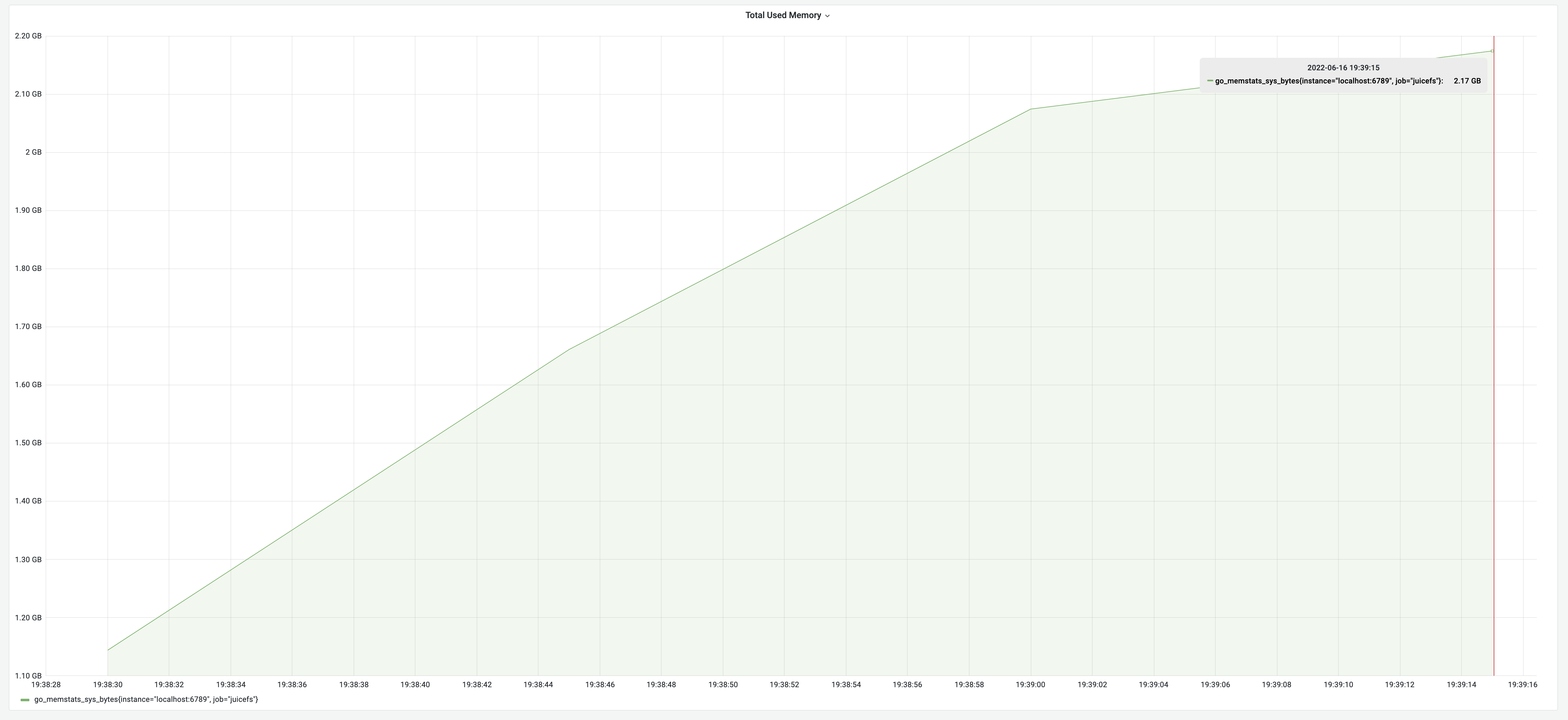
Performance after optimizing runtime
After implementing concurrent optimization, the test results showed a runtime of 1 minute, with memory usage of 2.17 GB. This brought a performance improvement of 125%.
Optimizing memory usage
How we optimized memory usage
Through the preceding tests, it became evident that memory usage optimization mainly focused on serialization efforts. The initial action of reading the entire JSON file and deserializing it into a structure demanded about twice the memory of the metadata, including the size of the JSON string and the size of the structure. Recognizing the substantial cost of reading the entire file, we adopted a streaming approach, reading and deserializing the smallest JSON object at a time. This significantly reduced memory usage.
Another concern during the load process was the storage of all entries in memory for recalculating nlink. This contributed significantly to high memory usage. The solution was straightforward: while nlink needed to be recalculated, it was unnecessary to record all attributes of an entry. By changing the value type of the map to int64, each insertion increased the value by 1. This eliminated the need for a large map, further reducing memory usage.
Performance after implementing streaming reads
With the implementation of streaming read optimization, the test results demonstrated a runtime of 40 seconds, with memory usage of 518 MB. The memory optimization achieved a remarkable improvement of 330%.
Performance after implementing streaming reads
Summary
Comparing JuiceFS 1.0-rc2 with v0.15.2:
- Dump process:
- Original: runtime of 7 minutes and 47 seconds, memory usage of 3.18 GB
- Optimized: runtime of 19 seconds, memory usage of 75 MB
- Improvement: 2300% in runtime, 4200% in memory usage
- Load process:
- Original: runtime of 2 minutes and 15 seconds, memory usage of 2.18 GB
- Optimized: runtime of 40 seconds, memory usage of 518 MB
- Improvement: 230% in runtime, 330% in memory usage
The optimization results were significant. We hope our experience will help you improve your optimization strategies and enhance your system performance.
If you have any questions or would like to learn more, feel free to join JuiceFS discussions on GitHub and our community on Slack.